
오늘 한 일은,
- SQL 공부
- [코드카타] SQL 9문제 풀기(149~157번)
- 머신러닝 공부
- [머신러닝 특강] "이상 탐지", "회귀" 수강하기
- [실무에 쓰는 머신러닝 기초] 1-8(차원 축소) , 1-9(이상 탐지) 실습하기
SQL 공부: [코드카타] SQL 문제 풀기(149~157번)
149. The PADS
Generate the following two result sets:
1. Query an alphabetically ordered list of all names in OCCUPATIONS, immediately followed by the first letter of each profession as a parenthetical (i.e.: enclosed in parentheses). For example: AnActorName(A), ADoctorName(D), AProfessorName(P), and ASingerName(S).
2. Query the number of ocurrences of each occupation in OCCUPATIONS. Sort the occurrences in ascending order, and output them in the following format:
"There are a total of [occupation_count] [occupation]s"
where [occupation_count] is the number of occurrences of an occupation in OCCUPATIONS and [occupation] is the lowercase occupation name. If more than one Occupation has the same [occupation_count], they should be ordered alphabetically.
SELECT CONCAT(name, '(', SUBSTR(occupation, 1, 1), ')') output
FROM occupations
ORDER BY output;

SELECT CONCAT('There are a total of ', oc.cnt, ' ', LOWER(oc.occupation), 's.') output
FROM (
    SELECT occupation,
           COUNT(occupation) cnt
    FROM occupations
    GROUP BY occupation
    ORDER BY cnt, occupation
) oc;
156. The Blunder
Samantha was tasked with calculating the average monthly salaries for all employees in the EMPLOYEES table, but did not realize her keyboard's key was broken until after completing the calculation. She wants your help finding the difference between her miscalculation (using salaries with any zeros removed), and the actual average salary.
Write a query calculating the amount of error (i.e.: 실제 평균 - 실수로 구해진 평균), and round it up to the next integer.
0을 제거하려면 어떻게 해야 하는지 기억이 안 나서 찾아봤다.
[참고] [Mysql] replace 문자열 치환 또는 변경! 해보자
- REPLACE(컬럼명, '찾을 문자', '변경할 문자')
SELECT ROUND(AVG(salary)) - ROUND(AVG(REPLACE(salary, '0', '')))
FROM employees
157. Top Earners
We define an employee's total earnings to be their monthly worked, and the maximum total earnings to be the maximum total earnings for any employee in the Employee table. Write a query to find the maximum total earnings for all employees as well as the total number of employees who have maximum total earnings. Then print these values as space-separated integers.
SELECT ee.earnings,
       COUNT(*)
FROM (
    SELECT employee_id,
           months*salary earnings
    FROM employee
    ORDER BY earnings DESC
)ee
WHERE earnings = (
    SELECT months*salary earnings
    FROM employee
    ORDER BY earnings DESC LIMIT 1
)
GROUP BY earnings
머신러닝 공부①: [실무에서 쓰는 머신러닝 기초]
이전에 공부한 머신러닝(차원 축소, 이상 탐지) 정리한 TIL:
[본캠프 40일차] SQL 공부, 머신러닝 공부
오늘 한 일은,SQL 공부[코드카타] SQL 7문제 풀기(138~144번)통계학 공부[통계 라이브세션] 6회차 수강하기머신러닝 공부[python standard] 9회차 수강하기[실무에 쓰는 머신러닝 기초] 1-6 실습하기[실무에
maandoo.tistory.com
차원 축소: [실습] PCA / t-SNE / UMAP으로 와인 데이터셋 차원 축소하기
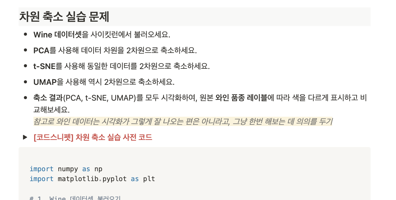
import numpy as np
import matplotlib.pyplot as plt

# 1. Wine 데이터셋 불러오기
from sklearn.datasets import load_wine
wine = load_wine()
X = wine.data
y = wine.target  # 3가지 와인 품종(0, 1, 2)
# 2. 차원 축소하기
from sklearn.decomposition import PCA
from sklearn.manifold import TSNE
from umap import UMAP
# PCA
pca = PCA(n_components=2)
X_pca = pca.fit_transform(X)
# t-SNE
tsne = TSNE(n_components=2, perplexity=30, random_state=42)
X_tsne = tsne.fit_transform(X)
# UMAP
umap = UMAP(n_components=2, n_neighbors=15, random_state=42)
X_umap = umap.fit_transform(X)
셋 다 동일하게 2차원으로 설정해주는데 t-SNE에선 perplexity를, umap에선 n_neighbors를 설정해줘야 한다. 일단은 배울 때 그냥 입력했던 대로 입력해서 우선 시각화해서 보기로 했다.
# 3. 시각화하기
fig, axes = plt.subplots(1, 3, figsize=(15, 4))

axes[0].scatter(X_pca[:, 0], X_pca[:, 1], c=y, alpha=0.7)
axes[0].set_title('PCA (2D)')
axes[1].scatter(X_tsne[:, 0], X_tsne[:, 1], c=y, alpha=0.7)
axes[1].set_title('t-SNE (2D)')
axes[2].scatter(X_umap[:, 0], X_umap[:, 1], c=y, alpha=0.7)
axes[2].set_title('UMAP (2D)')

plt.tight_layout()
plt.show()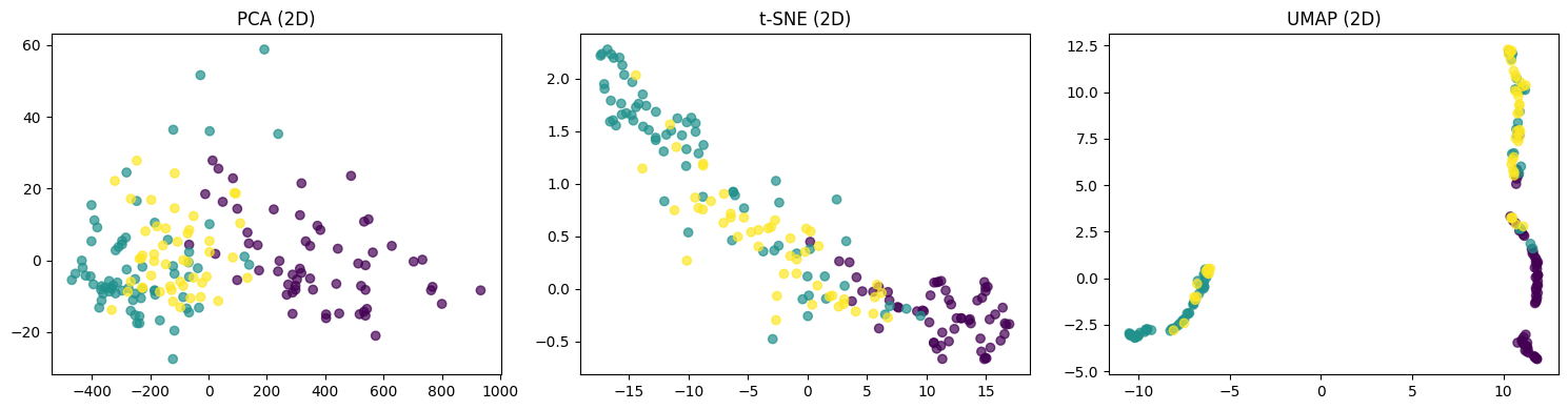
PCA, t-SNE는 그냥저냥 괜찮은 것 같기도 한데 확실한 건 UMAP은 진짜 이상하게 그려졌다.
t-SNE: perplexity 설정에 달라지는 시각화 확인하기
# 매개변수 조정하기
# t-SNE의 perplexity
perplexities = [5, 10, 20, 30, 50]
fig, axes = plt.subplots(1, len(perplexities), figsize=(20, 4))

for i, perp in enumerate(perplexities):
    tsne = TSNE(n_components=2, perplexity=perp, random_state=42)
    X_tsne = tsne.fit_transform(X)

    axes[i].scatter(X_tsne[:, 0], X_tsne[:, 1], c=y, alpha=0.7)
    axes[i].set_title(f"Perplexity = {perp}")

plt.tight_layout()
plt.show()

perplexities2 = [20, 25, 30, 40, 50]
fig, axes = plt.subplots(1, len(perplexities2), figsize=(20, 4))

for i, perp in enumerate(perplexities2):
    tsne = TSNE(n_components=2, perplexity=perp, random_state=42)
    X_tsne = tsne.fit_transform(X)

    axes[i].scatter(X_tsne[:, 0], X_tsne[:, 1], c=y, alpha=0.7)
    axes[i].set_title(f"Perplexity = {perp}")

plt.tight_layout()
plt.show()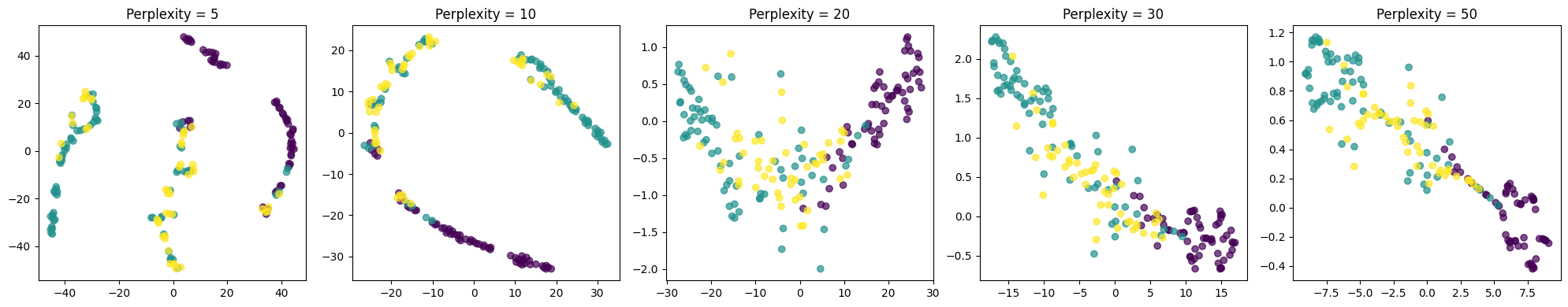

[참고1] t-SNE와 perplexity
[참고2] t-Stochastic Neighbor Embeddin (t-SNE)와 perplexity
[참고3] PCA, t-SNE 차원 축소(2)
일반적으로 t-SNE는 현재 데이터가 다차원일 때 2차원으로 축소해서 평면에 대략적으로 보기 위해 사용한다고 한다.
파라미터들 중 perplexity는 너무 높이면 거의 한 점처럼 보이고(작은 클러스터는 잘 안 보일 수 있음), 너무 낮으면 클러스터가 잘 되지 않는다(클러스터가 너무 세분화되어 사실 클러스터라 할 수 없는 상황일 수 있음). 기본값은 30이고 통상적으로 5~50 정도에서 설정한다고 한다.
그래서 perplexity의 값을 바꿔가면서 전부 시각화해봤는데, 주어진 와인 데이터셋을 2차원 시각화를 해보겠다면 한 25 정도로 설정해 그리면 될 것 같다.
UMAP: n_neighbors, min_dist 설정에 따라 달라지는 시각화 확인하기
[참고1] 210708목 - UMAP: Understanding UMAP 글 정리
[참고2] UMAP
UMAP은 t-SNE랑 비슷하지만 학습 속도도 빠르고, 군집 구조도 잘 보존해준다고 한다.
파라미터에서 중요한 것은 n_neighbors와 min_dist이다.
- n_neighbors: 각 클러스터에 포함하고자 하는 샘플의 개수 (기본=15)
값이 낮음 → 세부구조에 집중하도록 하여, 전체적인 구조를 해칠 수 있음
값이 높음 → 데이터의 전반적인 구조를 잘 반영하게 되는 대신, 세부적인 구조를 잃음 - min_dist: 샘플 간 거리의 최솟값 (기본=0.1)
값이 낮음 → 점들이 뭉쳐서 생성되어 클러스터링이나 더 세밀한 위상 구조 분석에 유용함
값이 높음→ 점들 서로를 밀집시키는 대신에 전체적인 위상 구조를 보존하는 데 초점을 둠
n_neighbors와 min_dist는 반비례 관계라고 한다.
# 매개변수 조정하기(2)
# UMAP의 n_neighbors와 min_dist

# 실험할 매개변수 값들
n_neighbors_list = [5, 15, 50]
min_dist_list = [0.0, 0.3, 0.9]

# subplot 설정
fig, axes = plt.subplots(len(n_neighbors_list), len(min_dist_list), figsize=(15, 12))

for i, n in enumerate(n_neighbors_list):
    for j, d in enumerate(min_dist_list):
        umap_model = UMAP(n_neighbors=n, min_dist=d, n_components=2, random_state=42)
        X_umap = umap_model.fit_transform(X)

        ax = axes[i][j]
        ax.scatter(X_umap[:, 0], X_umap[:, 1], c=y, alpha=0.7)
        ax.set_title(f"n_neighbors={n}, min_dist={d}")
        ax.set_xticks([])
        ax.set_yticks([])

plt.tight_layout()
plt.show()
...? 뭐가 좋은 걸까, 대체. 한 n_neighbors=5, min_dist=0.9 정도.....?
사실 잘 모르겠어, t-SNE도, UMPA도 시각화해서 뭘 보자는 건지...

이상 탐지: [실습] One-Class SVM / Isolation Forest로 와인 데이터셋에서 이상 탐지하기

import numpy as np
import matplotlib.pyplot as plt

# 1. Wine 데이터셋 로드
from sklearn.datasets import load_wine
wine = load_wine()
X = wine.data
y = wine.target

# 변수 2개만 선택 (예: 컬럼 0, 1)
X_2d = X[:, :2]  # shape: (178, 2)
feature_names = [wine.feature_names[0], wine.feature_names[1]]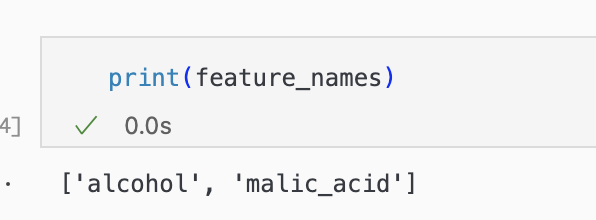
이번에도 산점도로 시각화해 볼 것이라서 어떤 컬럼들이 선택됐는지도 확인해봤다.
# 2. 이상 탐지하기
from sklearn.svm import OneClassSVM
from sklearn.ensemble import IsolationForest
# One-Class SVM
oc_svm = OneClassSVM(nu=0.05)
y_pred_oc = oc_svm.fit_predict(X_2d)
# Isolation Forest
iso_forest = IsolationForest(contamination=0.05, random_state=42)
y_pred_if = iso_forest.fit_predict(X_2d)

# 3. 이상치로 간주한 샘플 인덱스 추출
outliers_oc = np.where(y_pred_oc == -1)[0]
outliers_if = np.where(y_pred_if == -1)[0]

print("=== One-Class SVM ===")
print("이상치로 탐지된 샘플 개수:", len(outliers_oc))
print("이상치 인덱스:", outliers_oc)

print("\n=== Isolation Forest ===")
print("이상치로 탐지된 샘플 개수:", len(outliers_if))
print("이상치 인덱스:", outliers_if)
One-Class SVM이랑 Isolation Forest로 이상 탐지를 위해 하는데 매개변수는 그냥 수업 속에서 진행했던 대로 그냥 똑같이 뒀다.
이상치로 간주된 데이터의 개수와 인덱스를 출력해서 보니, 개수는 둘 다 9개를 이상치로 간주했는데 7개는 동일한데 나머지 2개는 모델에 따라 다른 값이 나왔다.
# 4. 이상치 시각화하기
fig, axes = plt.subplots(1, 2, figsize=(12, 5))

axes[0].scatter(X_2d[:, 0], X_2d[:, 1], label='Normal')
axes[0].scatter(X_2d[outliers_oc, 0], X_2d[outliers_oc, 1], color='tomato', edgecolors='k', label='Outliers')
axes[0].set_title('One-Class SVM')
axes[0].set_xlabel(feature_names[0])
axes[0].set_ylabel(feature_names[1])
axes[0].legend()

axes[1].scatter(X_2d[:, 0], X_2d[:, 1], label='Normal')
axes[1].scatter(X_2d[outliers_if, 0], X_2d[outliers_if, 1], color='tomato', edgecolors='k', label='Outliers')
axes[1].set_title('Isolation Forest')
axes[1].set_xlabel(feature_names[0])
axes[1].set_ylabel(feature_names[1])
axes[1].legend()

plt.tight_layout()
plt.show()
'[내배캠] 데이터분석 6기 > 본캠프 기록' 카테고리의 다른 글
| [본캠프 45일차] 심화 프로젝트 준비 (0) | 2025.04.21 |
|---|---|
| [본캠프 44일차] 심화 프로젝트 준비 (0) | 2025.04.18 |
| [본캠프 41일차] SQL 공부, 머신러닝 공부 (1) | 2025.04.15 |
| [본캠프 40일차] SQL 공부, 머신러닝 공부 (0) | 2025.04.14 |
| [본캠프 39일차] SQL 공부, QCC ④, 머신러닝 공부 (0) | 2025.04.11 |